Handwritten notes on risk assessment with formulas for risk aversion, ride seeking, and risk neutral, showing various mathematical symbols and variables.

To plot an individuals EU on a graph, we also need to find the value for the X axis (income), so we use this simple formula:

Handwritten physics equation showing Einstein's mass-energy equivalence: E equals mc squared.

This article is based on a research paper by Gary Becker linked here.

Because criminals can weigh the cost and benefits of their crime* Gary Becker was able to derive a formula for crime:

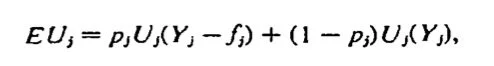
Close-up of a mathematical formula written in black ink.

which means EU (satisfaction) = probability of being caught (p) x utility of income after punishment* (Y -f) + probability of not being caught (1-p) x utility of income not being caught (Y). This is to find the value for the Y axis.

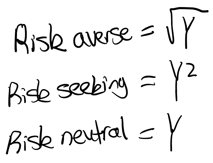
Where the utility function is dependent on whether an individual is:

When we plot the answers to this equation on a graph, it looks like this:

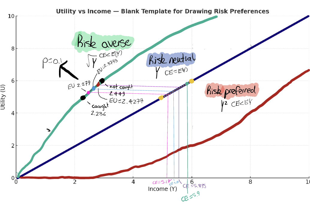
Graph comparing utility vs income with three curves labeled risk averse, risk neutral, and risk preferred. Data points and notes on calculations are shown, illustrating different risk preferences.

As you can see:
Risk averse - concave curve
Risk seeking - convex curve
Risk neutral - linear (benchmark)

To see why the curves are concave, convex and linear, let’s go through one calculation, and see where it lands.

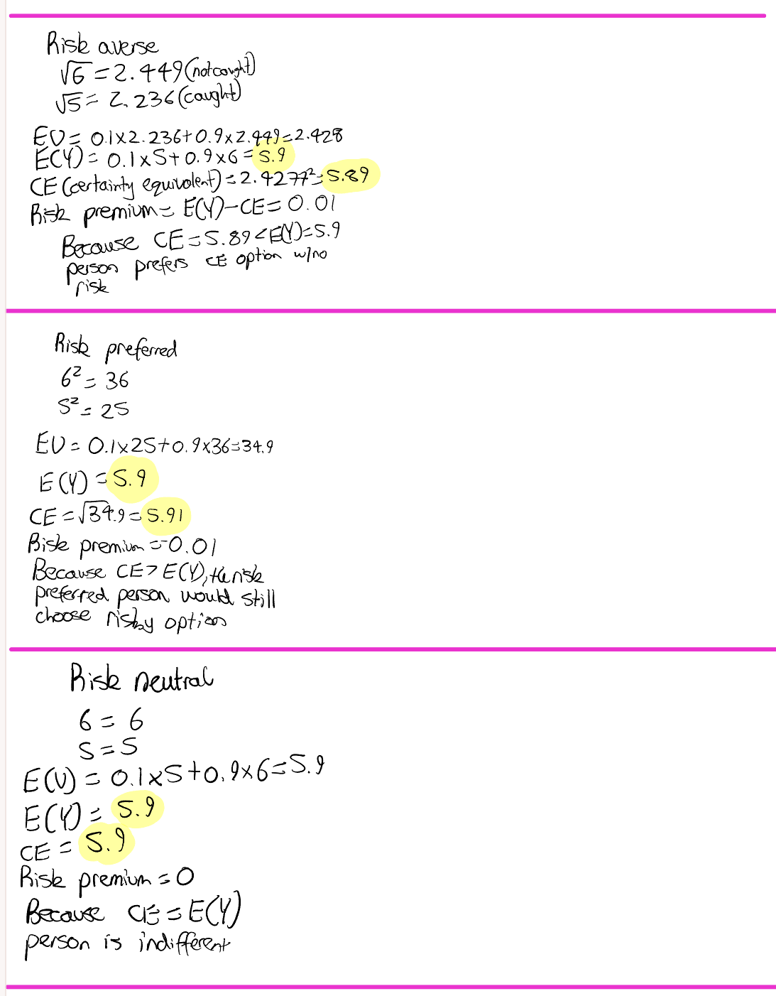
For risk averse:
Let’s say the probability of being caught (P) is = 0.1. Then let’s say:
Income not caught = $6
Income caught = $5 (to keep it simple)

Because we know the two possible outcomes, we can create a sort of boundary of possibilities, with certainty that our EU (satisfaction) will lie somewhere in between. To do this, we square root our income values (remember, for risk averse = always square root, for others, it changes)

Income if not caught = square root of 6 = 2.449 (upper “boundar” - represented by black dot)
Income if caught = square root of 5 = 2.236 (lower “boundary” - represented by black dot)

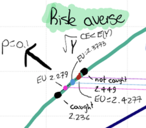
Hand-drawn graph showing risk aversion. It includes labels for 'people', 'not caught', and 'caught', with corresponding numerical values, and features mathematical symbols like square root and Euclidean distance. The graph is shaded in green and some lines are in purple.

Again, these two black dots are our two possible outcomes, showing the EU:
-> individual not caught = benefit (EU) is 2.449
-> individual caught = benefit 2.236

The average satisfaction (expected utility) lies between these two dots. Below I calculated the expected utility (EU) and expected income, so we could plot our dot.

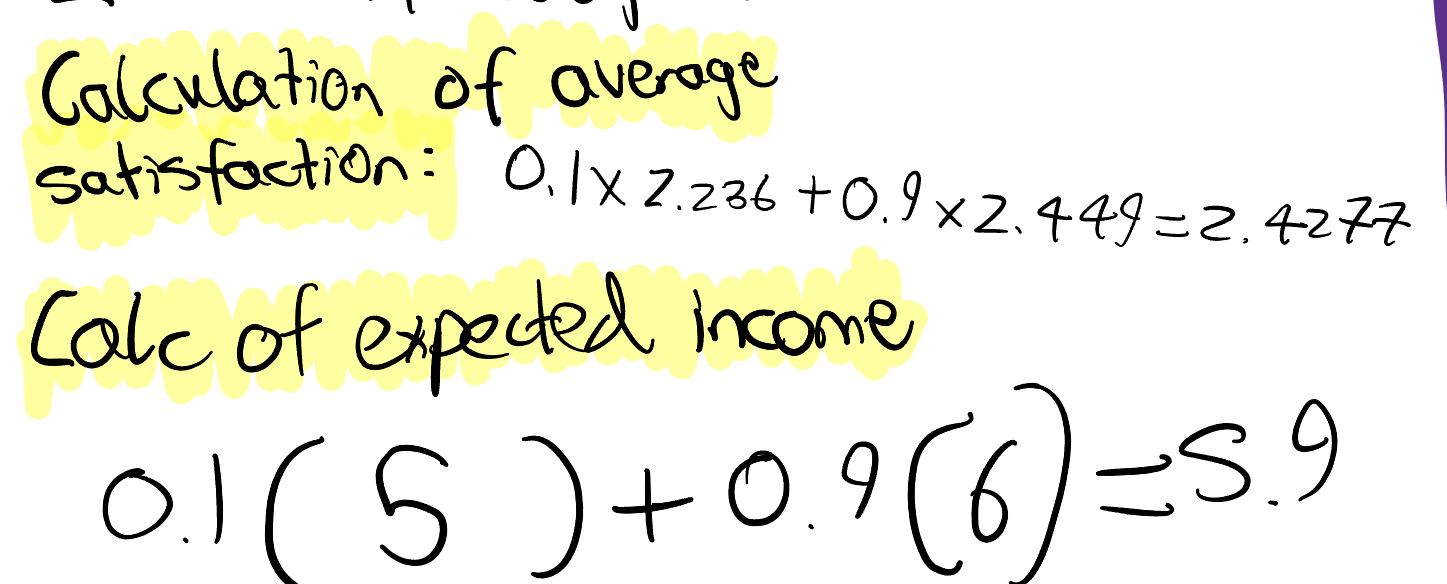
Handwritten notes with calculations for average satisfaction and expected income, highlighted with yellow background.

A graph titled 'Utility vs Income — Blank Template for Drawing Risk Preferences' shows three utility curves labeled 'Risk averse' in green, 'Risk neutral' in blue, and 'Risk preferred' in red. The green curve is convex, the blue is straight, and the red is concave. The graph includes data points, equations, and notes about certain expected utility values and risk calculations.

The answer was 5.9, 2.4277 - therefore we graph that on the x and y axis.
As shown on the graph, it is very close to the “not caught” outcome - this is because the probability of being caught was 0.1 - so obviously it is close to the not caught outcome when graphed.

Additionally, when you draw a horizontal line from it to the risk neutral line, and then draw another line downwards (or just do 2.428^2), you get 5.89 - which is called the certainty equivalent (CE). This how much one values their stolen money.

For risk averse, the CE (5.89) is less than the expected income (5.9) for risk neutral, which means this individual is risk averse. So the risk averse individual would accept less to avoid risk.

However, for a risk preferred individual, I calculated their CE (5.91) to be greater than the expected income (5.9) for risk neutral. This means they are risk preferred. They would need to be compensated to give up risk.

And for a risk neutral, their CE of 5.9 is = their E(Y) of 5.9. They are indifferent.

Increasing p, all else equal:
When we use all the same variables but increased p to 0.8, our dot/answer moves closer to the caught outcome and reduces the EU to 2.279.

Increasing f, all else equal
However, what happens when we reduce the income if caught (and keep p at 0.1)? The dot/answer moves closer to the not caught outcome and reduces the EU to 2.3773.

In summary: an increase in either p or f reduces the EU, and moves the dot closer to the caught outcome. Makes sense - an increase in policing or an increase in punishment is likely to reduce crime.

REFERENCES:
Full disclosure, ChatGPT was used to help me understand risk averse/preferred/neutral and to fact check - however, it was not used to write anything or perform calculations.

Becker, Gary. “Chapter Title: Crime and Punishment: An Economic Approach Crime and Punishment: An Economic Approach.” National Bureau of Economic Research, vol. ISBN, 1974, pp. 0–87014, www.nber.org/system/files/chapters/c3625/c3625.pdf.

In Case of Econ Struggles. “Master Expected Utility in under 4 Minutes.” YouTube, 24 Sept. 2024, www.youtube.com/watch?v=Ho4fsiNHcdo. Accessed 11 Oct. 2025.

Iris Franz. “Expected Utility (1): Risk Aversion, Risk Loving, and Risk Neutral.” YouTube, 11 Oct. 2019, www.youtube.com/watch?v=cSZvSy4Vopc. Accessed 11 Oct. 2025.

Silz-Carson, Katherine. “Expected Utility and Risk Preferences.” YouTube, 22 Sept. 2020, www.youtube.com/watch?v=xjJBepUMkfE.

CALCULATIONS