
Cournot Duopoly, Quantity Competition: The Optimal Quantity, Balancing Market Share & Profitability
References quoted & linked below
Game theory analyses situations for individuals/entities using games. A game is a situation in which decisions are interdependent, creating a shared, mutual impact and is displayed on a “matrix". The combination of each “player’s” decision results in a payout, otherwise known as utility. Typically the higher the number the higher the utility.
5 Minute Read
Per (Liberto), taking the expected market supply of a competitor into consideration, two firms in this duopoly market model SIMULTANEOUSLY chooses the quantity that presents the ‘best response’ to the competitor’s production quantity. The product produced is homogenous. They are essentially competing for market share through quantity produced, a key difference to Bertrand competition, in which firms compete in prices.
Continuing with (Liberto), the amount selected to produce is important, because according to the law of demand, there’s an inverse relationship between quantity and price (higher qty = lower price, vice versa), thus there’s a trade off: produce more, but have the price lower, or produce less, and have the price rise. So what’s the Nash equilibrium, that is, what’s a stable amount of goods produced no other firm will deviate from?
Definition of Cournot Duopoly
Consider a Duopoly market with two firms, Riley Inc (A) and Sadie Inc (B).
Intuition: Producing one unit of the homogenous product costs $4.5. The intercept is 10, meaning if nothing was produced, the maximum willingness to pay would be 10, and for each extra unit produced by Riley or Sadie Inc, the price in the market falls by $1.
Workings
Riley Inc = A, Sadie Inc = B
Cournot Model; The Quantity Competition:
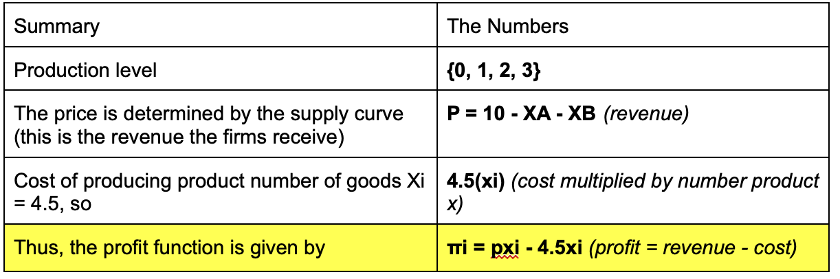
The following is the dynamic between supply and price:
10 - XA - XB
This is NOT a payoff matrix.
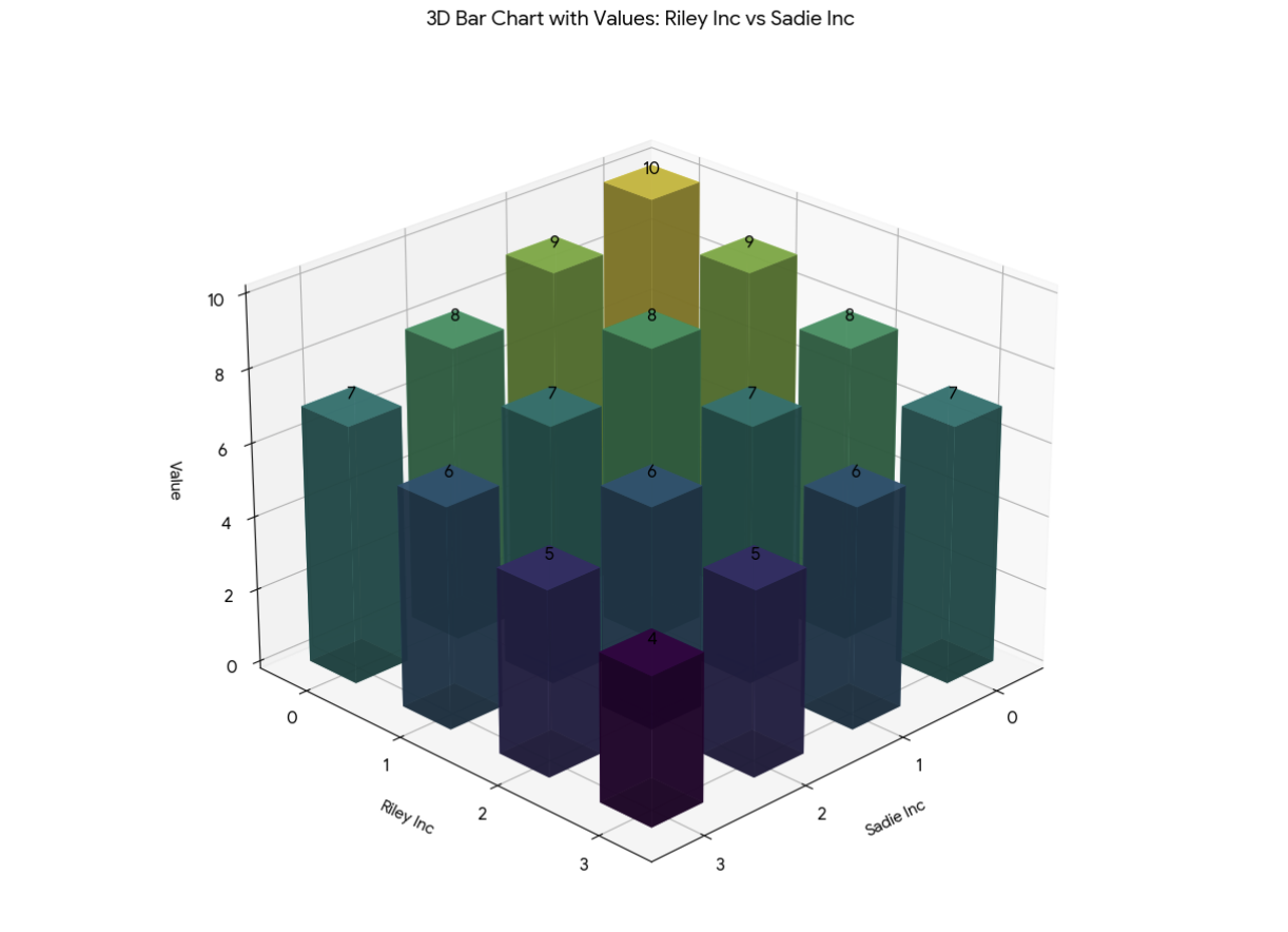
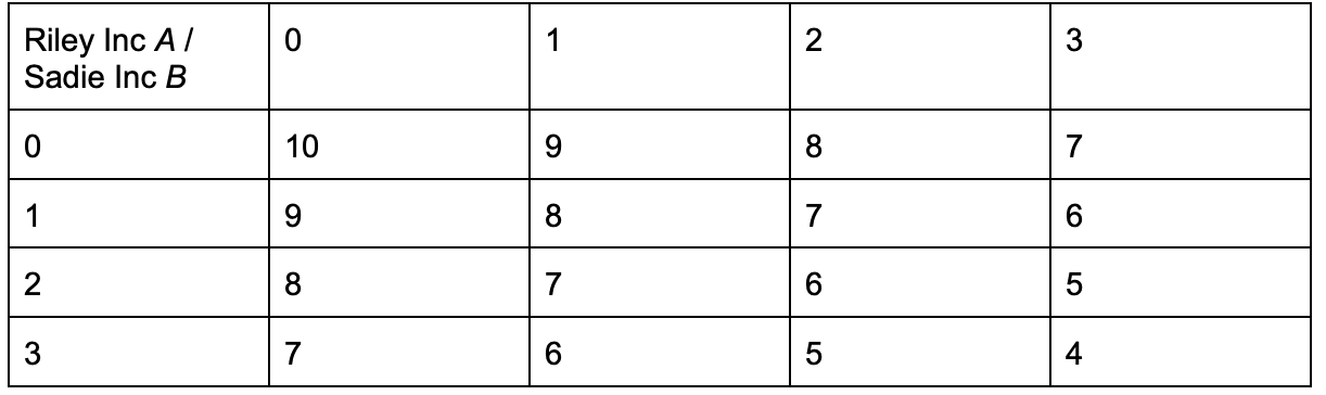
If we look at both extremes: production at 0 and production at 3, the price in this market is 10 and 4 respectively. The price would be 10 at a production level of 0 because everyone would be demanding the good, and the price would be bid up. Conversely, the price would be 4 at a production level of 3 because there would be more goods than people demand, so the price would be bid down.
This lines up with the law of demand that explains that “the quantity purchased varies inversely with price.” (Hayes) Remember; both firms simultaneously decide to produce, say, 1 each of the product (quantity) and the price in the market will be 8, because price = 1 - 1 = 8 (P = 10 - XA - XB)
Monopoly, Cournot, Perfect Competition
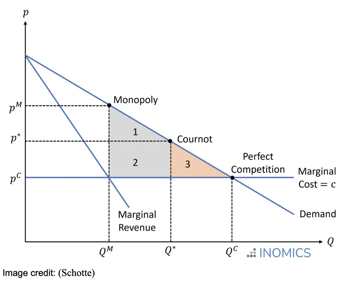
Above you can see market quantities and prices made under a monopoly, Cournot duopoly and perfect competition, in order.
In a perfectly competitive market, price = marginal cost and firms earn zero profits, thus pC = a - bQC = c. But because firms in cournot firms earn profits, we can conclude that the total quantity produced is lower and the price is higher than in the competitive market equilibrium. (Schotte) In a monopoly (single seller), less is produced, and more profits are made- this is not a stable equilibrium, so it cannot be a cournot duopoly. Thus, cournot sits in the middle. (Hayes, “What Is a Monopoly? Types, Regulations, and Impact on Markets”)
Areas 1+2 illustrate the welfare gain with cournot monopoly, whereas area 3 illustrates the deadweight loss created by cournot competition compared to perfect competition. “ Antoine Cournot argued that by colluding and forming a cartel, the two firms in the market could move toward the monopoly solution.” (Schotte) But the monopoly solution isn’t stable. If both collude and decide to produce 1 both earning 3.5, one may want to increase profit by producing 2, so it will deviate and earn 5 whilst the other earns 2.5. So, what is the Nash equilibrium? We can find it by looking at the payoff matrix. (Schotte)
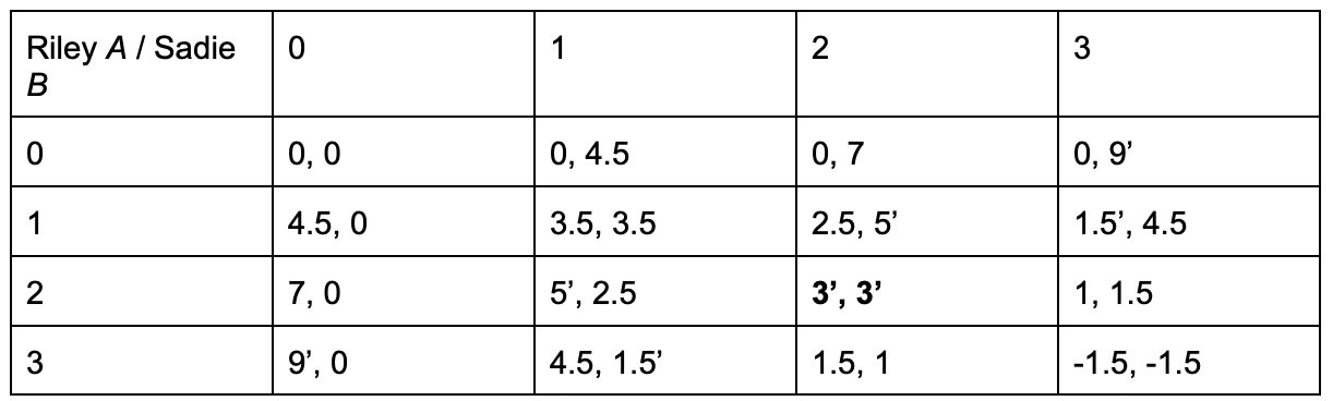
The Payoff Matrix
This is the payoff matrix: each payoff is derived by: pxi - 4.5xi (revenue - cost)
For example, if XA = 1 and XB = 3 the price is 6 (=10 - 1 - 3).
Riley (A) (6 -4.5) x 1 = π = 1.5
Sadie (B) (6-4.5) x 3 = π = 4.5
Nash equilibrium (NE): The NE here is (2,2), both earning a profit of 3. This is the equilibrium where neither will deviate, it is mutually beneficial- the best response to the other player’s responses… a balance between production levels and profit.
Strategy 1,1
This strategy earns each player 3.5, “so why isn’t this the equilibrium?”
This is not the Nash equilibrium because both players will deviate. Riley Inc would rather choose production level 2 (5>3.5), and Sadie Inc would choose production level 2 (5>3.5).
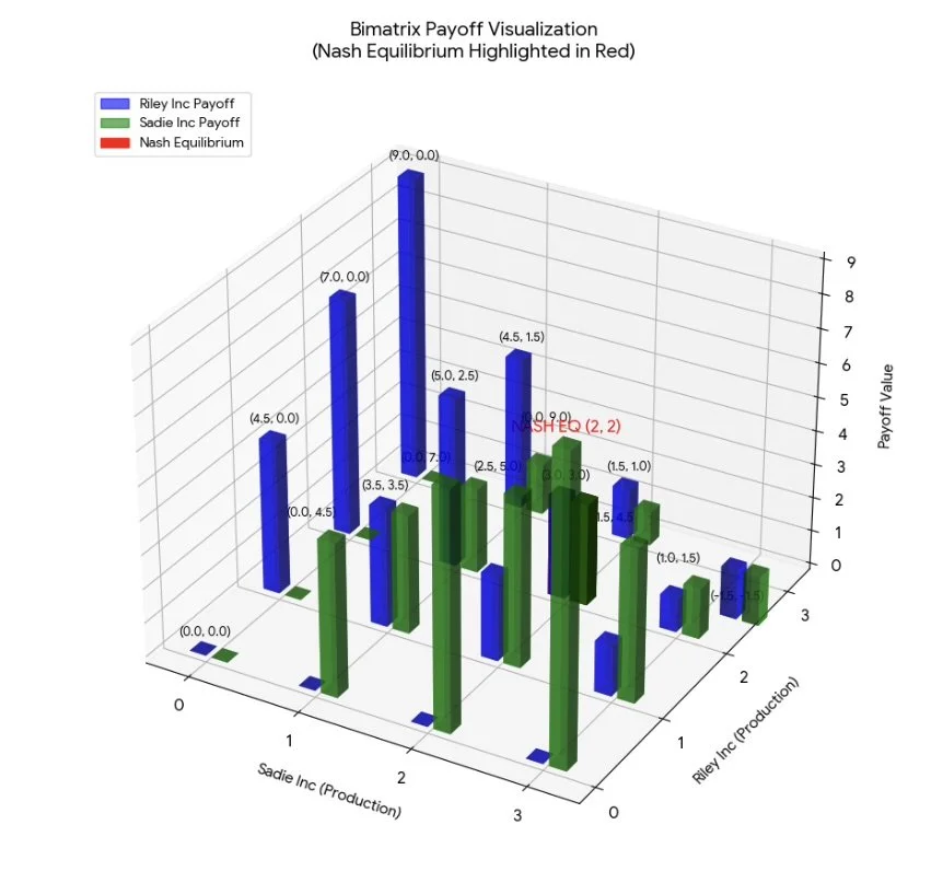
This is the payoff matrix visualised (Bimatrix). The nash equilibrium is highlighted in red.
Would Riley Inc still choose XA = 2 if Sadie Inc went bankrupt?
No, because Riley Inc could produce 3 and earn 9 - price is not disrupted by the extra supply because Sadie Inc isn’t producing anything.(Suzuki)
OPEC, the Organisation of the Petroleum Exporting Countries (OPEC) is considered to be an oligopoly, setting production quotas (quantity) to maximise profits and market share. (Liberto)
Example
Per (Liberto) some drawbacks of the Cournot model include (but not limited to):
1. In a duopoly, it’s more realistic to say firms are responsive to each other’s quantity changes. The classic cournot model simply assumes the two firms choose quantities independent of each other.
2. The model’s critics question how firms compete on quantity rather than price. “The suitability of price rather than quantity as the main variable in oligopoly models was confirmed in subsequent research by several economists.” (Liberto)
3. It’s difficult to have a product that is completely homogenous.
4. Assuming two companies have identical cost structures is a big assumption (author’s opinion)
Drawbacks of Cournot Model
Cournot duopoly is a model of two firms with similar costs, selling homogenous products. The businesses try to maximise sales volume (market share) and higher prices (more profits). Whilst the Cournot model has drawbacks, the Cournot method improves both market share and profitability by defining an optimum quantity (although not Pareto optimal). The Cournot Duopoly game shows price and quantity between monopolistic levels (low output, high prices) and perfectly competitive levels (high output, low prices) (when market participants increase). Cournot provides the Nash equilibrium where no firm will deviate. (Yes, collusion is possible but it’s fragile). OPEC is considered to be a cournot oligopoly, setting production quotas (quantity) to maximise profits and market share.
Summary
References
“Game Theory II: Cournot Duopoly | Policonomics.” Policonomics.com, policonomics.com/lp-game-theory2-cournot-duopoly-model/.
Hayes, Adam. “Organization of Petroleum Exporting Countries (OPEC).” Investopedia, 10 July 2022, www.investopedia.com/terms/o/opec.asp.
---. “What Is a Monopoly? Types, Regulations, and Impact on Markets.” Investopedia, 21 June 2024, www.investopedia.com/terms/m/monopoly.asp.
---. “What Is the Law of Demand in Economics, and How Does It Work?” Investopedia, 11 May 2025, www.investopedia.com/terms/l/lawofdemand.asp.
Liberto, Daniel. “Cournot Competition.” Investopedia, 31 Oct. 2021, www.investopedia.com/terms/c/cournot-competition.asp.
Schotte, Simone. “Cournot Competition.” INOMICS, 31 May 2022, inomics.com/terms/cournot-competition-1525473.