
Perfectly Competitive Markets
You Can’t Set the Price,
So What Can You Do? -
Liam Scotchmer
TABLE OF CONTENTS
Definition
Rundown
Features of Perfectly Competitive Markets
How Price Is Determined In a Perfectly Competitive Market
Demand & Supply Curves
Cost Curves for an Individual Firm
Profit Maximisation Rule
How Much Profit?
Short Run vs Long Run Decisions
Profit Is Driven To Zero
Demand and Supply Shifting
What Does Zero Profit Mean?
Limitations
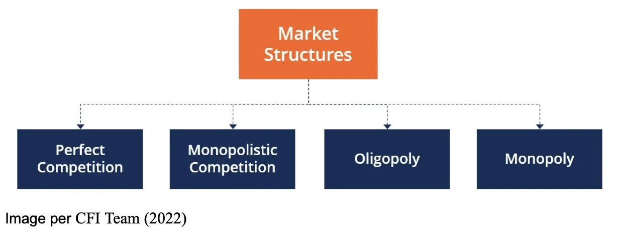
Perfect competition is a theoretical benchmark economists use, a sort of blueprint for supply and demand dynamics. Other market structures like monopolistic competition, oligopolies and monopolies can be compared to it.
Whilst it is a theoretical model, some industries come close to it, for example; commodities (oil, gold), farming (bananas, wheat, rice), FOREX, shares, Bitcoin and more. (Gans et al.)
Definition
The question is: firms in a perfectly competitive market are price takers, so how do they maximise profit, and when do they decide to shut down, exit, or keep producing?
The goal of any firm is to maximise profit: typically, like many markets (monopolistic competition, oligopolies) firms can product differentiate or set prices to do so. However, a defining feature of a perfectly competitive market is firms cannot set prices or product differentiate. In other words, firms are price takers, not price makers. This is a brutal market, one where efficiency matters! (hint: when no profit or losses are made, firms produce where marginal cost equals the minimum average total cost of production, called at efficient scale).
Graphically a firm’s (individual) demand curve is horizontal/perfectly elastic, the price is fixed! Demand is equal to marginal revenue = average revenue = price.
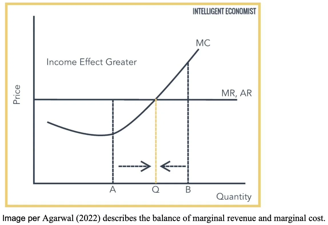
With a horizontal demand curve/fixed price, firms exclusively have output as their lever for profit maximisation; which means equating the appropriate output to produce that balances marginal revenue and marginal costs*.
*The marginal cost curve also equals the upward sloping supply curve.
Marginal costs can be split into average variable costs (AVC) and average fixed costs (AFC).
In the short run, marginal revenue (price) covering variable costs matters only (fixed costs matter in the long run). Aside from the firm's own financial decisions, the ability to ensure P is greater than AVC is determined by many factors, like consumer demand. Demand can fluctuate, shifting the demand curve up or down, and with it price, andaffect the amount of profit firms make. If the price goes below AVC, firms will shut down. Alternatively, if the price is above AVC, firms can stay.
In the long run, both fixed and variable costs matter, called average total cost (ATC). Firms decide whether to enter or exit the market entirely: if the price is above ATC other firms will enter, or if the price is below ATC, firms will exit. This long term enter/exit dynamic shifts the supply curve endlessly until any economic losses or profits that were made in the short run have been reduced to zero (so now MR = MC).
The cause of zero economic profit in a perfectly competitive market? Low barriers to entry.
When do firms shut down? When P < AVC (shutdown point).
When do firms exit? When P < ATC.
When do firms keep producing? When P > AVC.
Rundown
Per Hayes (2025);
1) Buyers and sellers are so numerous that each on its own has little impact on the market price
2) as buyers and sellers accept the given market price, they are all called price takers.
3) the goods being sold are homogenous or a commodity
4) firms can exit/enter the market without cost
5) prices are determined solely by supply and demand, therefore companies earn just enough profit to stay in business, and no more.
Further
6) buyers have complete/perfect information about the product being sold
7) capital resources and labour are perfectly mobile (efficiency- resources can be reallocated instantly to where they’re most needed and workers are employed in a field that is most suited to them)
(Hayes)
Main Features of a Perfectly Competitive Market
How Price Is Determined In a Perfectly Competitive Market
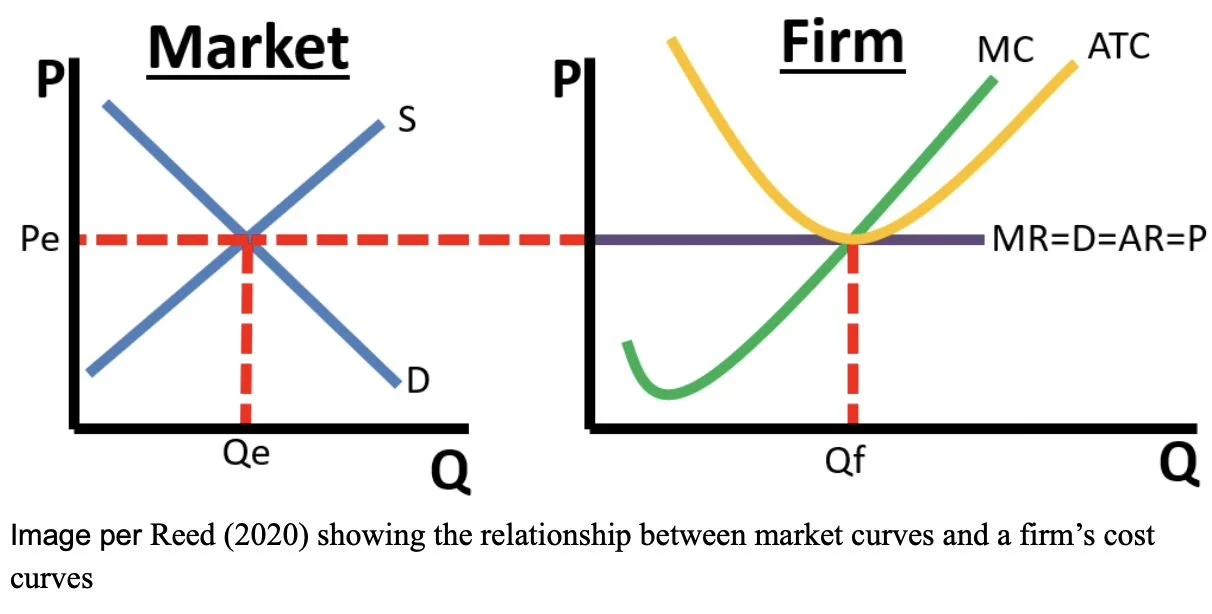
The intersection of supply and demand is the price firms in a perfectly competitive market sell their goods/services at. (Gans et al.) Therefore, price is decided by market supply and demand and not individual firms (this is seen in the first graph).
As explained later, the curves shift from changing demand and supply (exit/entry).
Demand & Supply Curves
Demand Curve
In the first graph, the market as a whole has a downward sloping demand curve, obeying the law of demand (e.g. higher prices decreases total quantity demanded). (Gans et al.) However, in the second graph, the demand curve for a firm is horizontal because each firm is too small to move the market price. The demand curve is also equal to marginal revenue, average revenue, and price (MR=D=AR=P) (explained next).
Supply Curve
Pictured above, per Gans et al (2021), in the first graph, the supply curve is upward sloping. This is because the marginal cost curve is also upward sloping (due to the law of diminishing returns). The two curves are related! Firms supply only the quantity where MR = MC.
Cost Curves For an Individual Firm
We’ve explained the supply and demand curves for a market and firm, now the cost curves for an individual firm:
MR = D = AR = P, per Gans et al. (2021) because:
1) demand curve horizontal at market price (horizontal because firm is too small to move the market price)
2) MR = P (because selling one more unit never changes price)
3) average revenue AR = R(Q)/Q = P, mathematically
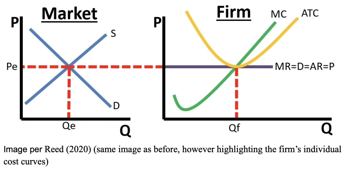
Marginal Cost (MC) curve:
U shaped due to the law of diminishing returns (more input = less output eventually, so production output is diminishing and therefore more costs are required -> MC up)
MC = MR
MC crosses MR, and firms produce at that quantity (profit maximisation rule, explained next) (Gans et al.)
ATC
Average Total Cost (ATC) curve, U shaped due to falling fixed costs, and then rising variable costs. (Gans et al.)
Key Takeaway:
1) firms produce where MC equals MR (but may shutdown or exit if making a loss, as explained later).
2) Average total cost curve crosses MC curve at its minimum point, called at “efficient scale” whereby the quantity of output minimises average total costs. (Gans et al.) MC should cross ATC at the minimum point because companies must be able to competitively price in such a competitive market. (Tardi)
3) P = MR = AR = D where price is set by market supply and demand (not by the firm).
Price Takers Vs Price Makers
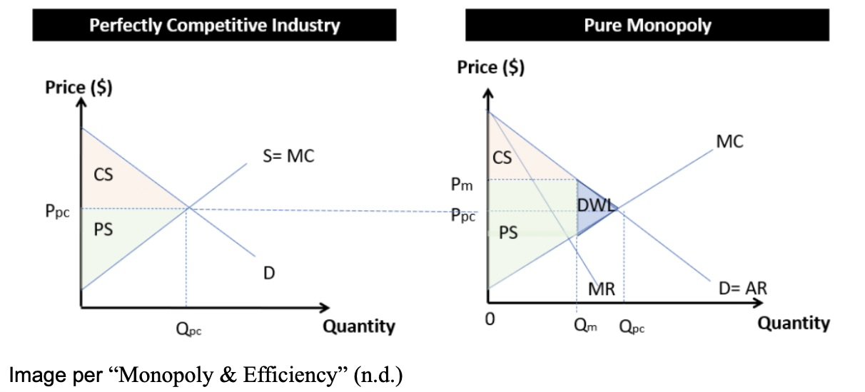
It’s important to note that “the relation between marginal revenue and the quantity of output produced depends on market structure.” For a perfectly competitive firm, marginal revenue = price = average revenue. On the other hand, for a monopoly, monopolistic competition or oligopoly firm, marginal revenue is less than average revenue and price because these firms must sell at a lower price to generate another sale (why? this is explained at the end). (“AmosWEB Is Economics: Encyclonomic WEB*Pedia”)
The goal of any firm, per Gans et al. (2021) is to maximise profit, and does so by maximising the difference between revenue and cost. But how do firms in a perfectly competitive market do so if they are price takers?
As firms are unable to decide price (they are price takers), they can only decide:
Quantity of output (for profit maximising)
Entry/Exit (explained later)
Firms in a perfectly competitive market choose how much to produce! They equate the appropriate quantity to produce that balances marginal revenue (MR) and marginal cost (MC), meaning if MR is not equal to MC, they will adjust output.
MC > MR = Firm is making a loss on the last unit produced = reduce output, costs lower, back to MR = MC.
MC < MR = Firm is making a profit on the last unit produced = increase output, costs rise. back to MR = MC.
This is called profit maximisation, and the equilibrium is where MR = MC.
Profit Maximisation Rule (MR = MC)
At the end are limitations of the profit maximisation rule.
The firm maximises profit when it produces Q*, but how large is this profit?
To find out, let’s adjust our graph so it represents this question:
How Much Profit?
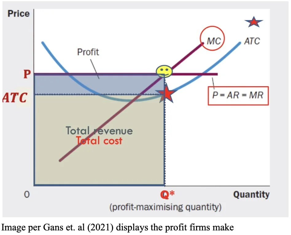
Profit = (P-ATC) x Q
Profit is equal to market price minus average total cost times by quantity. However, as we will see next, profit can be made in the short run but not in the long run.
Graphed:
- MC = MR = P which determines profit maximising Q* (P is also = AR & MR)
- The star is the ATC of producing profit maximising Q*
- Profit is difference; the area of the blue rectangle
Short Run vs Long Run Decisions
Average total cost is equal to average fixed cost plus average variable cost (or ATC = AFC + AVC).
Short Run - Shutdown/Stay
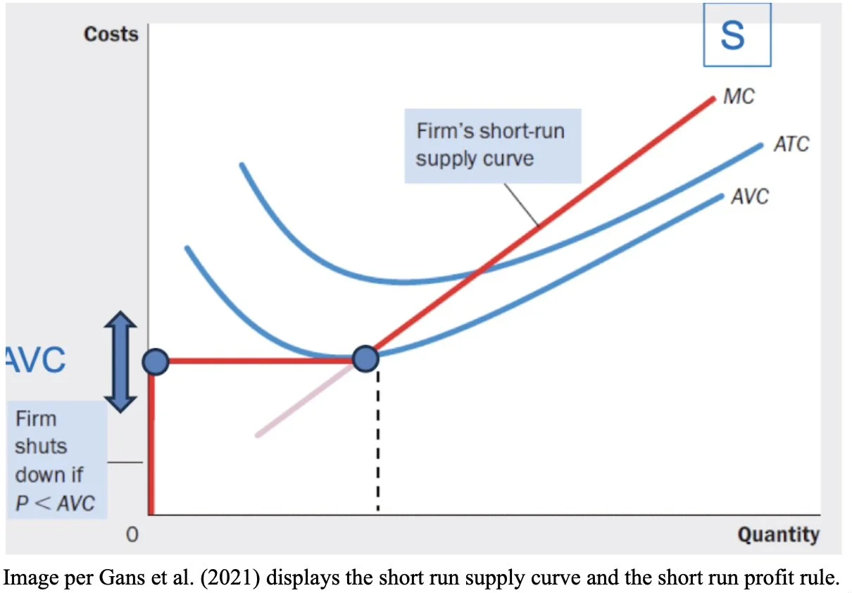
Per Gans et al. (2021), in the short run, there is a fixed number of firms, so firms cannot simply enter or exit the market so quickly or easily. Additionally, firms only care about variable costs as fixed costs are “sunk costs.”
Firms choose to either shut down or stay depending on price and average variable cost.
P > AVC = stay (as fixed costs are sunk, they don’t matter in the short run)
P < AVC = shutdown
Per Gans et al. (2021) a “firm’s short run supply curve starts at P = AVC and then coincides with MC.”
The graph below shows the short run rule:
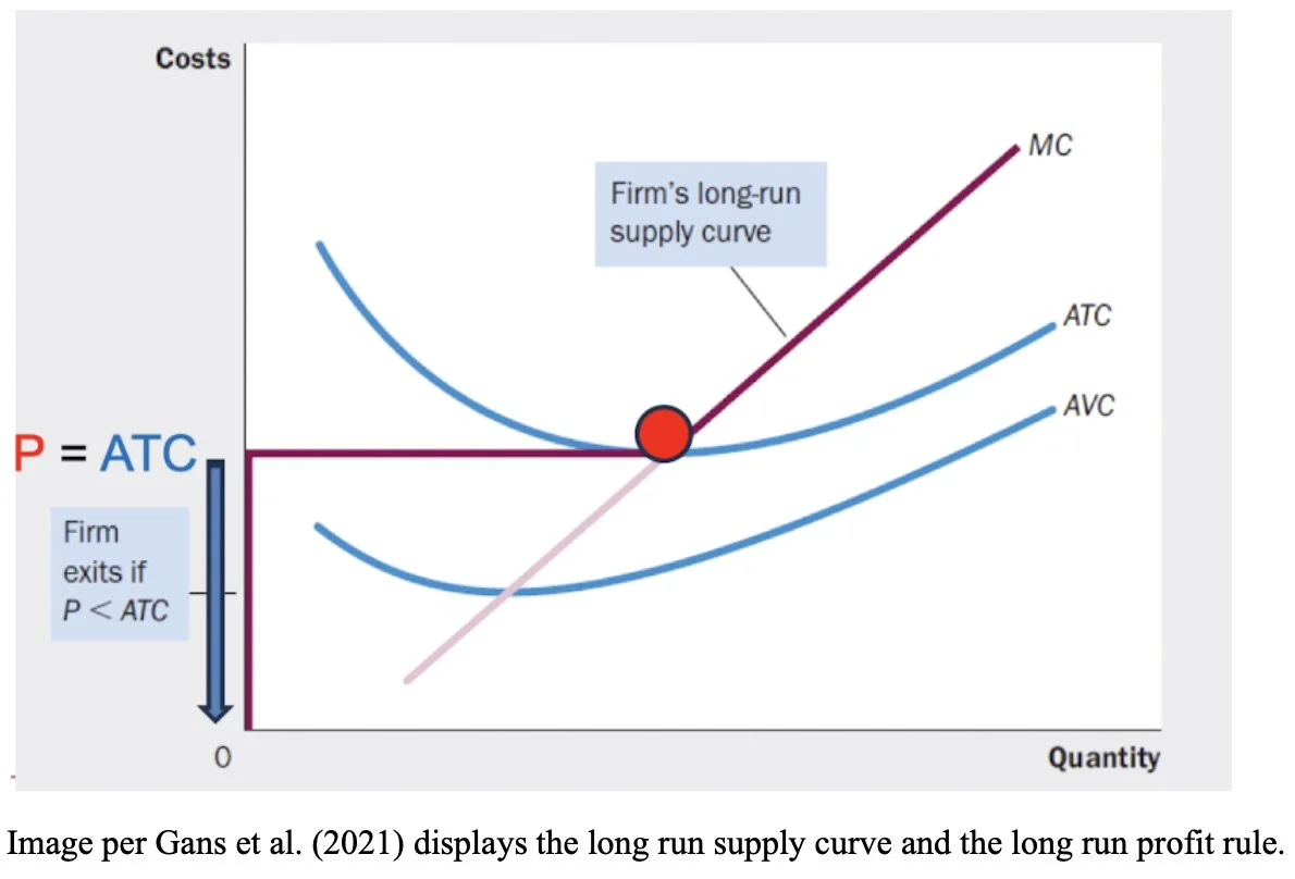
Long Run - Exit/Enter
Shutdown or stay is a short-run decision to produce nothing for a specific period of time.
However, exit or enter is a long-run decision to leave the market entirely. (Gans et al.)
Exiting or entering a market is a decision made as a long run decision based on both variable costs and fixed costs (fixed costs are no longer sunk costs).
Therefore, the firm exits when P < ATC.
A firm enters when P > ATC.
The equilibrium is where P = ATC, as explained next.
(Gans et al.)
Per Gans et al. (2021) a “firm’s long run supply curve starts at P = ATC and coincides with MC.”
The graph below shows this rule.
Profit Is Driven To Zero
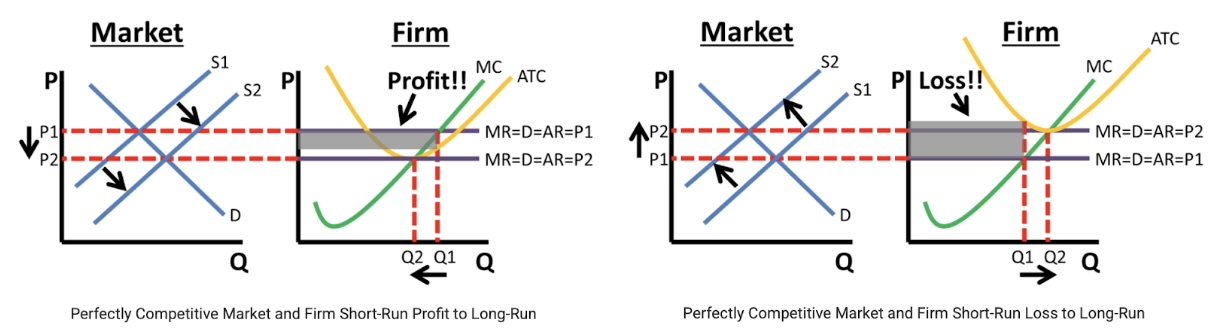
In a competitive market, there are low barriers to entry. This makes it facile for the market supply curve to shift in the long run. For example, per Reed (2020):
Market earning profit: In this case, firms/entrepreneurs will be attracted by the profit, and will enter the market -> the market supply curve will shift to the right -> market price will decrease and MR=D=AR=P. Economic profit goes to zero all in the long run.
Market earning a loss: In this case firms exit the market, shifting the supply curve to the left, increasing the price and MR=D=AR=P until the firm breaks even. Economic profit goes to zero all in the long run.
Market earning zero: process of entry/exit ends.
“ In the end, low barriers to entry (and exit) mean competitive markets earn zero economic profit in the long run. “ (Reed)
Remember, firms cannot exit or enter the market in the short run, this only occurs in the long run. Therefore, economic profit can be made briefly in the short run. (Reed)
Profit or loss is the area of the rectangle: length is Q and height is P-ATC.
This also means that in the long run, ATC = MC and therefore operate at their efficient scale, or in other words, the market price is equal to the minimum average total cost of production. Read further here.
Per Gans et. al (2021), demand and supply can shift.
Demand shifting: if demand increases, causing the demand curve to shift right, the price in the market will rise. In the short run firms will enjoy an increase in profits, but with free entry into the market, those profits will attract new competitors.
Supply shifting: if supply increases due to demand increasing, this entry of firms shifts the supply curve to the right and the price drops. This occurs in the long run. Economic profits are zero.
Demand & Supply Shifting
What Does Zero Profit Mean?
Per Gans et al. (2021), zero economic profit does not mean zero earnings. “Firms stay in business with zero economic profit because revenue still covers all opportunity costs, including the owner’s time and capital.”
For example, if the total opportunity cost of owning a farm is $80,000/year, and the farm is earning $80,000:
Economic profit = 0
Accounting profit = $80,000
Limitations
Limitations of Profit Maximisation Rule (MC=MR)
Per Agarwal (2022) limitations of the profit maximisation rule include:
1) in the real world it is difficult to calculate the revenue and costs of the last product sold, e.g. it is hard for firms to know the price elasticity of demand for their goods, which determines the MR.
2) The profit maximisation rule also depends on how other firms react (if every firm decides to increase prices, demand will be inelastic, but if only one firm does so, demand will be elastic)
3) Isolating the effect of changing the price on demand is difficult. Demand could change to many factors other than price.
4) Higher prices could attract new firms to enter the market, so firms may pursue less than maximum profits and higher market share.
Limitations of Perfect Competition
Whilst perfect competition is a useful structure for comprehending how supply and demand impact prices and behaviour in a market economy, it differs from reality.
Product Differentiation
Stating that the “goods are homogenous” collapses for two reasons: product differentiation is a marketing strategy to encourage consumers to choose one product/brand over another and is commonly employed by companies to stand out. (Kopp) Secondly, with almost every product, there is variation. (Hayes)
Perfect information
Having complete/perfect information about a product is difficult in real life, and whilst “consumer awareness has increased with the information age” there are still few industries where consumers have complete information about all products and sellers. (Hayes).
Barriers to Entry
Stating that firms can enter and exit without cost is unrealistic: there are barriers to entry such as high startup costs or strict government regulations. (Hayes)
Capital Resources and Workers are Perfectly Mobile
Capital resources that can be reallocated instantly to where they’re most needed, also known as Pareto Efficiency implies there is perfect competition and resources are used to the maximum level of efficiency without at least one being made worse off. This is difficult to achieve, and again, it assumes perfect competition, which is rare. It is also hard to imagine a world in which all workers can be employed in a field that is most suited to them- underemployment exists.
References
Agarwal, Prateek. “Profit Maximization Rule.” Intelligent Economist, Intelligent Economist, 2 Feb. 2022, www.intelligenteconomist.com/profit-maximization-rule/.
“AmosWEB Is Economics: Encyclonomic WEB*Pedia.” Amosweb.com, 2026, www.amosweb.com/cgi-bin/awb_nav.pl?s=wpd&c=dsp&k=marginal+revenue%2C+perfect+competition. Accessed 26 Feb. 2026.
Analyst Prep. “Price, Marginal Cost, Marginal Revenue, Economic Profit, and the Elasticity of Demand.” AnalystPrep | CFA® Exam Study Notes, 24 Sept. 2021, analystprep.com/cfa-level-1-exam/economics/price-marginal-cost-marginal-revenue-economic-profit-and-the-elasticity-of-demand/.
CFI Team. “Market Structure.” Corporate Finance Institute, 23 Apr. 2022, corporatefinanceinstitute.com/resources/economics/market-structure/.
Economics Help A-Level. “Monopoly Diagram - Explanation and Efficiency.” YouTube, 17 Nov. 2025, www.youtube.com/watch?v=T-Tn_HfP54E. Accessed 26 Feb. 2026.
Gans, Joshua, et al. Principles of Microeconomics. South Melbourne, Victoria, Australia, Cengage Learning Australia, 2021.
Hayes, Adam. “Perfect Competition: Examples and How It Works.” Investopedia, 31 May 2025, www.investopedia.com/terms/p/perfectcompetition.asp.
Indeed Editorial Team. “Average Revenue Formula: Definition and Example.” Indeed Career Guide, 2025, www.indeed.com/career-advice/career-development/average-revenue-formula.
Lumen Learning. “Profit Maximization in a Perfectly Competitive Market | Microeconomics.” Courses.lumenlearning.com, 2022, courses.lumenlearning.com/wm-microeconomics/chapter/profit-maximization-in-a-perfectly-competitive-market/.
“Monopoly & Efficiency.” Economics Tuition SG, economics-tuition.sg/monopoly-efficiency/.
“Reading: Price and Revenue in a Perfectly Competitive Industry and Firm | Microeconomics.” Lumenlearning.com, 2012, courses.lumenlearning.com/suny-microeconomics/chapter/price-and-revenue-in-a-perfectly-competitive-industry-and-a-perfectly-competitive-firm/.
Reed, Jacob. “Keys to Understanding Perfectly Competitive Markets.” ReviewEcon.com, 24 Sept. 2020, www.reviewecon.com/perfect-competition.
Tardi, Carla. “Why Minimum Efficient Scale Matters.” Investopedia, 3 Oct. 2021, www.investopedia.com/terms/m/minimum_efficiency_scale.asp.
Tse, Harry. “Lecture 2. Firms in the Competitive Market.” 2026.
Tuovila, Alicia. “Marginal Revenue Explained, with Formula and Example.” Investopedia, 17 June 2024, www.investopedia.com/terms/m/marginal-revenue-mr.asp.