
When Is Doing More Worth It?
Microeconomics 2nd Year
15 Minute Read
TABLE OF CONTENTS
Accounting Vs Economic Profit
The Production Function
Marginal Product
Marginal Product of Labour
Cost Function
Marginal Cost
Why Production Typically Exhibits Diminishing Marginal Product
Diminishing Marginal Product and Marginal Costs
Average Total Costs in Short Run
Average Total Costs in Long Run
Returns To Scale
Profit Maximising Rule
Real World Application
Profit Maximisation For A Monopoly
Firms should only expand production while the marginal benefit exceeds the marginal cost, and diminishing marginal product ensures that this condition eventually fails….
The Fundamental Point;
Though an oversimplification, the aim of firms is to maximise profit. (Kenton, “What You Should Know about Firms”) Profit is calculated by total revenue (TR) minus total cost (TC). This is not done by increasing total revenue alone.. this is also done by increasing the difference between total revenue and total cost. (Gans et al.) (Later on, we discuss that firms can maximise profits if it produces at an output where marginal revenue (MR) = marginal cost (MC)).
The Aim of Firms
Accounting Profit Vs Economic Profit
Profit can be measured as economic profit or accounting profit. Accounting profit is where explicit costs are included only, that is, out of pocket expenses, so total revenue - explicit costs.. On the other hand, economic profit includes explicit AND implicit costs. Implicit costs are the options / choices forgone. Economic profit is total revenue - explicit - implicit costs, and is therefore always smaller than accounting profit because it introduces another cost to factor in. (Hargrave)
Explicit costs can be variable (ie. wages) and/or fixed costs (ie. rent).
Implicit costs “offers insight into the efficiency of a company by considering alternative uses of resources” and are good for long term decision making. (Hargrave) Continuing with Investopedia (Hargrave), for example, selling a natural resource for the market price versus utilising that resource: selling on the market for some revenue is the forgone option, and that revenue from the market is therefore an implicit cost.
Per (Tse, Tutorial 1: The Costs of Production (Questions)), Economists like to use functions to express inputs, like costs and revenue and their relationship with output, ie.: production.
On the graph below, you can see the production function, 20L - 2L², which shows how output changes as labour changes. The production function is important because it shows us that as input increases, output rises at first, then eventually falls due to diminishing returns. (Tse, Lecture 1 - Production and Costs - Economics for Business 2)
The Production Function
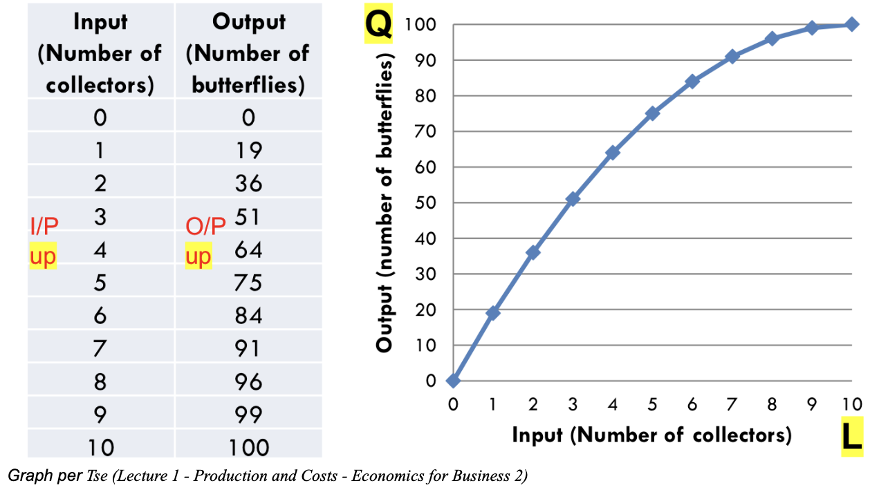
Per Whiteley (2026), the negative 2L² tells us it’s an upside down parabola. They are trying to show how output decreases as input increases in an exponential relationship of Q=20L-2L².
Why the Negative 2L²?
Economists/companies don’t look at total product, they look at marginal product, the “additional output created as a result of additional input placed into the company.” (Masterclass B) Eg.: the additional coffees (output) made at a cafe as a result of hiring one additional employee (input).
Again, marginal product is the additional output created as a result of additional input placed into a company. (MasterClass) Marginal product is the derivative of the production function.
Per MasterClass (2020), to accurately measure marginal product, one must isolate a specific input and its change and then track how that change increases output (derivatives!)
The inputs businesses can isolate are, for example, labour! (others include land, capital, and raw materials).
Marginal Product (MP)
Applying Marginal Product
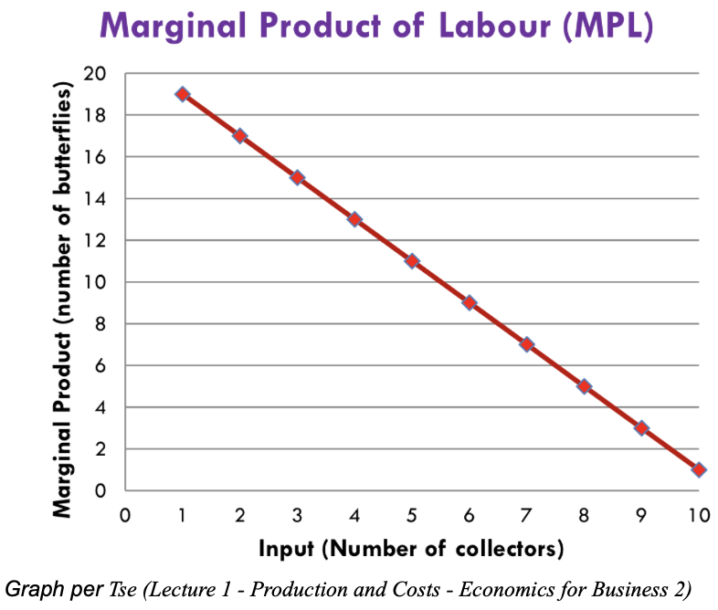
Now that we understand marginal product, we can isolate one input: labour. This is called marginal product of labour (MPL), and is the extra output from one more worker. It is downward sloping as seen below because, as stated by the law of diminishing returns, in the short run, investment in a production input (ceteris paribus) “will yield increased marginal product, but as the business scales up each additional increase of a production input will yield progressively lower increases in output.” (Masterclass) This can be due to overcrowding, inefficiencies, and not enough space. (“Law of Diminishing Marginal Productivity”)
Marginal Product of Labour (MPL)
From Production Function to Cost Function

Total cost represents both fixed costs (rent, permits) plus variable costs (wages, raw material). In the short run, at least one cost is fixed, but in the long run, all costs are variable.
Fixed costs (FC) do not change with output, e.g. 10.
Variable costs (VC) change with output, e.g. 10Q.
(Gans et al.)
Example (optional read)
This example is per Tse, Lecture 1 - Production and Costs - Economics for Business 2 (2026)
Assume that for a firm producing binders, total costs are given by the function:
TC(Q) = 10 + 2Q + 0.5Q^2
1. What are the total costs (TC) if the firm produces 20 binders? And what are the fixed (FC) and variable costs (VC)?
TC = 250 : (10+2(20)+0.5(20)^2
FC = 10
VC = 240
2. Using the same function as above, write down the equation for the average total cost (ATC) and calculate the ATC if the firm produces 20 binders.
ATC/Q = 250/20 = 12.5
3. Plot the TC curve and ATC curve
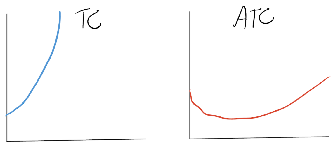
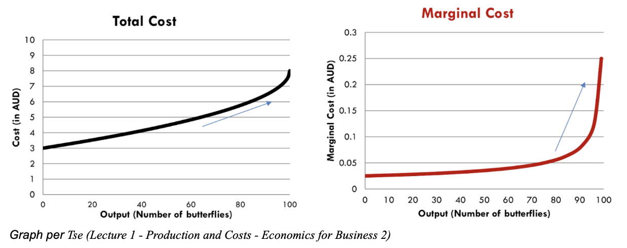
Total cost (TC) curve - total costs rise when output rises because of diminishing marginal product causing marginal cost to rise.
Average total cost (ATC) - is a per unit cost, per “Total Cost vs Average Cost vs Marginal Cost” (2025). It is a U shape as it begins high as variable costs are high when output is low (imagine wage costs compared to little output), but starts to fall because fixed costs are spread over more output. However, it eventually rises and forms a U shape because of diminishing marginal product, that is, inefficiency! Marginal costs spike, or more specifically, the variable cost curve rises causing ATC to rise overall. (Gans et al.)
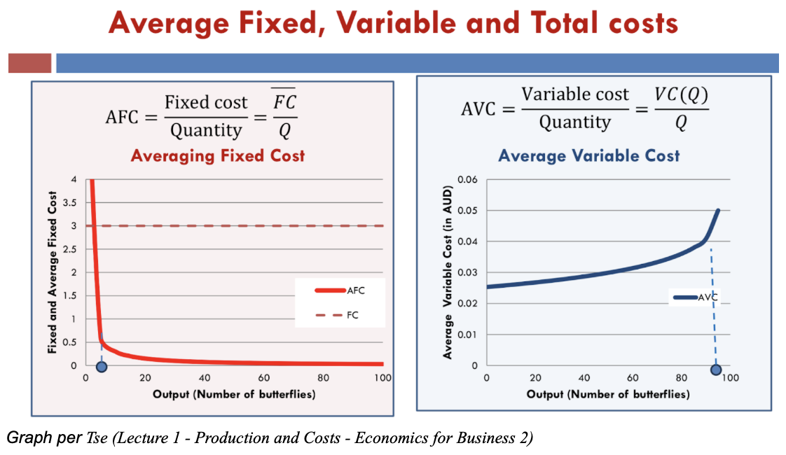
The below graph illustrates the differences between TC, FC and VC curves.
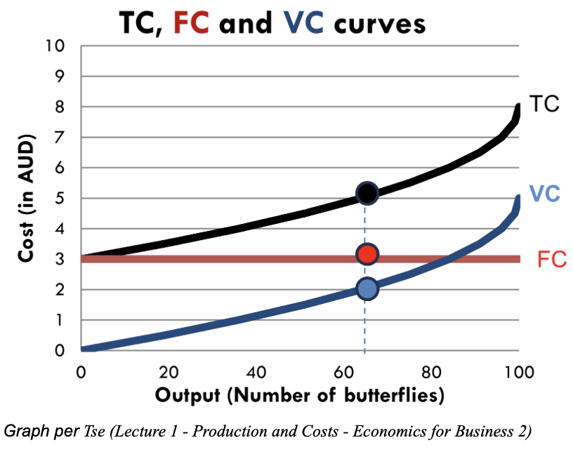
TC is FC + VC.
“Marginal cost (MC) is the increase in total cost (TC) caused by an extra unit of production (Q)” (Gans et al.), or in other words, it is the cost of one additional unit.
Properties: The marginal cost curve rises rapidly with the amount of output produced, reflecting the property of diminishing marginal product, as explained below. (Gans et al.)
You can see the total cost curve versus the marginal cost curve side by side below.
Marginal Cost
Why Production Typically Exhibits Diminishing Marginal Product
Diminishing marginal product, using marginal product of labour (MPL) as an example, occurs when each additional worker adds less extra output as more labour is added. (Gans et al.)
MPL goes down as labour rises.
This happens because; in the short run, some inputs (capital, machines, space) are fixed, and as more workers are added, workers share the same machines, workspaces become crowded, and efficiency falls. Each worker produces less additional output. (“Law of Diminishing Marginal Productivity”)
Read the next section to see why diminishing marginal product causes marginal costs to rise.
Diminishing Marginal Product and Marginal Costs
Diminishing marginal product, whereby output grows at a fast rate initially, and eventually but ultimately grows at a declining rate, means more (variable) costs are needed when expanding production. This explains why marginal costs rise dramatically. (“Law of Diminishing Marginal Productivity”)
Important to note: Per Gans et al. (2021), in the short run, many costs are fixed (at least 1) because, for example, increasing the number of machines or space in a short amount of time is not possible.
Continuing with Gans et al. (2021):
Average total cost is the average of fixed and variable costs (= ATC/Q).
In the short run:
- Average fixed costs (per unit) fall as output rises because fixed costs are spread over many units -> AFC is always downward sloping (= AFC/Q)
- Average variable costs (per unit) are costly when output is low, and also costly when output is high -> AVC is U shaped (= AVC/Q)
Average Total Costs in Short Run
(next; in the long run)
-> Thus, both AFC and AVC combined, the average total cost curve is U shaped.
-> MC curve crosses ATC at the lowest point because if MC is greater than ATC, ATC rises, and if MC is lower than ATC, ATC falls. The medium is called at "efficient scale” (at the quantity of output that minimises ATC). For example, per Tse (2026), if your average mark is 80, and you receive a new mark of 70, your average mark will fall. Conversely, if your new mark is 90, your average mark will rise.
As said by Gans et al. (2021), in the long run, fixed costs become variable costs.
Average total costs in the long run are bound by 3 properties:
Economies of Scale
Meaning: in the long run, as the firm gets bigger, the cost per unit decreases. This can happen due to marketing, spreading fixed costs, or bulk buying. (Kenton)
Diseconomies of Scale
Opposite of economies of scale, meaning; in the long run, average total cost rises as output increases. This increase in cost when output rises can happen due to raw material price changes, shortages of goods, interest rate increases, or other economic influences. (Investopedia)
Constant Returns To Scale
Meaning: cost per unit stays the same as the firm expands. For example, if a soap manufacturer doubles its total input (100->200), and its output also doubles (1000->2000), it has achieved constant returns to scale. (Majaski)
Average Total Costs in Long Run
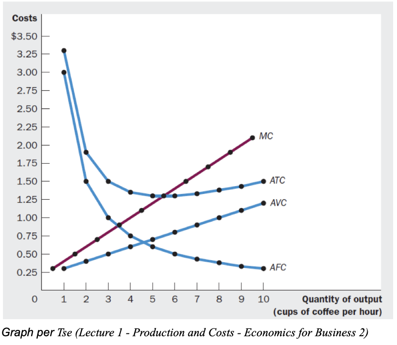
All Cost Curves Combined
As you can see (intuition per Gans et al.):
AFC falls as output rises because fixed costs are spread over many units.
AVC rises as output rises because of diminishing marginal product, which means inefficiency, and thus results in more (variable) costs needed in the production process.
ATC is U shaped because it is a combination of AFC and AVC.
MC rises with the amount of output produced, reflecting the property of diminishing marginal product, whereby inefficiencies arise (less productivity in production process so more workers are needed i.e. variable costs) and marginal costs rises.
MC = MR (the crossing) is important, this is the profit maximising rule (explained next).
The following is per Fiveable Content Team (2025)
Marginal revenue (MR) equals the marginal cost. This is the profit maximising rule. This applies to all types of firms, whether they are in PC, MC, oligopoly, or monopoly. (Remember, marginal cost meaning the cost of the last unit produced. We are comparing marginal costs to marginal revenue).
The profit maximising point for firms is where MR = MC (however doesn’t mean the company is making a profit) because in disequilibrium:
MR > MC, firms will produce more when MR > MC because they are making extra profits, until price falls from extra supply and MR = MC.
MR < MC, firms will produce less when MR < MC because they will be making a loss and reduce output, until supply falls and prices are bid up and MR = MC.
“The profit maximisation rule states that a firm maximises its profit by producing the quantity of output where marginal revenue (MR) equals marginal cost (MC).” (Fiveable Content Team) This ensures that companies “do not produce too little or too much, ultimately leading to optimal resource allocation” (in terms of profit).
Profit Maximising Rule
Example of MR & MC
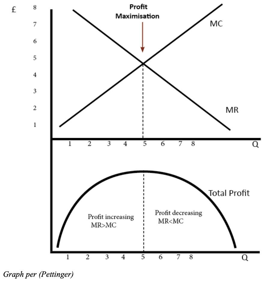
Example per Pettinger (2019):
For example, looking at the diagram above, if the firm produces an output less than 5, MR is > MC. Therefore, for this extra output, the firm is gaining more revenue than it is paying costs, and total profit will increase.
At an output of 4, MR is only just greater than MC, so the firm is still making a profit.
At an output greater than 5, the marginal cost will be greater than marginal revenue and the firm will be at a loss.
Occurrence
MR > MC occurs when fixed or variable costs rise, causing the firm to lower production to maintain profitability.
MR < MC may occur if for example, technology reduces production costs, allowing firms to produce more at a lower cost, “allowing them to expand output while still adhering to the Profit Maximisation Rule.” (Fiveable Content Team)
In perfect competition, firms are price takers, thus marginal revenue equals the market price! This makes it easy to apply this profit maximisation rule since firms adjust their output based on market prices. However, in a monopoly, output is still set where MR = MC but prices are charged higher than in perfectly competitive markets. This means marginal revenue is less than price “due to the downward sloping demand curve.” (Fiveable Content Team) (they mean that when prices rise, demand falls, therefore to sell more, prices must fall, so marginal revenue is less than price, MR < P). (AI was used to help me understand just this last part).
A bottled air company (in a perfect market) can produce nothing, so output = 0: it will have fixed costs to pay (rent, insurance), but variable costs are zero.
However, the company’s CEO, along with many other companies, commences operations with 20 workers bottling air on the production floor.
She notes a few things (in short run!):
1) average fixed costs per unit produced fell as output rose.
2) average variable costs per unit are high to begin with, but as workers begin to produce more bottles, the variable costs become more manageable. The average variable cost falls with productivity rising. Cost per unit falls.
The CEO is now looking at increasing the employees who bottle air, but notices the amount produced per worker falls. This is diminishing marginal product of labour (less output per extra worker). She notes this is due to the production floor becoming crowded, and miscommunications causing errors in order destinations. Less orders are being completed.
This is a perfect example of productivity falling! Workers are producing less, so now the CEO must hire more workers per extra unit causing marginal costs to rise. In other words, marginal costs (from wages, a variable cost) are rising due to inefficiencies- diminishing marginal product.
This explains 4 things:
Marginal cost rises because of diminishing marginal product.
Average fixed cost falls because fixed costs are spread over many units.
Average variable costs are high initially, but begin to fall as output rises, however then they rise back up due to diminishing marginal product.
Average total cost forms a U shape as AFC falls, and AVC rises.
MR = MC
In this perfectly competitive market (air is a commodity), the firm adjusts their output based on market price. However, because costs are rising, MR < MC,the company is producing too much relative to the profit max point. The company reduces output (fires workers), so do many other companies who have recently entered the market who are in a similar situation. This reduction in supply, market wide, causes prices to rise as supply is less than demand. So MR = MC again, and therefore, the company has correctly chosen the output where profit is maximised.
Real World Application
Profit Maximisation For A Monopoly
ChatGPT. Used for discussion and clarification of microeconomic concepts and structural feedback only; not used to generate or write the article When Is Doing More Worth It? (2026).
“Average Cost.” Wikipedia, 7 Jan. 2020, en.wikipedia.org/wiki/Average_cost.
Economics Help A-Level. “Monopoly Diagram - Explanation and Efficiency.” Youtu.be, 2026, youtu.be/T-Tn_HfP54E. Accessed 22 Feb. 2026.
Fiveable Content Team. “Profit Maximization Rule (MR = MC) - (AP Microeconomics) - Vocab, Definition, Explanations | Fiveable.” Fiveable.me, 2025, fiveable.me/key-terms/ap-micro/profit-maximization-rule-mr-=-mc. Accessed 2025.
Gans, Joshua, et al. Principles of Microeconomics. South Melbourne, Victoria, Australia, Cengage Learning Australia, 2021.
Hargrave, Marshall. “How Do Economic Profit and Accounting Profit Differ?” Investopedia, 30 Oct. 2024, www.investopedia.com/ask/answers/033015/what-difference-between-economic-profit-and-accounting-profit.asp.
Investopedia. “Understanding Diseconomies of Scale.” Investopedia, 1 Jan. 2021, www.investopedia.com/terms/d/diseconomiesofscale.asp.
Kenton, Will. “Economies of Scale: What Are They and How Are They Used?” Investopedia, 30 May 2025, www.investopedia.com/terms/e/economiesofscale.asp.
---. “What You Should Know about Firms.” Investopedia, 2019, www.investopedia.com/terms/f/firm.asp.
“Law of Diminishing Marginal Productivity.” Monash Business School, www.monash.edu/business/marketing/marketing-dictionary/l/law-of-diminishing-marginal-productivity.
Majaski, Christina. “Understanding Diminishing Marginal Returns and Returns to Scale.” Investopedia, 2025, www.investopedia.com/ask/answers/033015/whats-difference-between-diminishing-marginal-returns-and-returns-scale.asp#toc-exploring-returns-to-scale-constant-increasing-and-decreasing. Accessed 22 Feb. 2026.
MasterClass. “Economics 101: What Is Marginal Product? Learn How to Calculate Marginal Product and Its Impact on Business - 2024 - MasterClass.” MasterClass, 2020, www.masterclass.com/articles/economics-101-what-is-marginal-product.
Masterclass B. “Economics 101: What Is Marginal Product? Learn How to Calculate Marginal Product and Its Impact on Business - 2024 - MasterClass.” MasterClass, 2020, www.masterclass.com/articles/economics-101-what-is-marginal-product.
Pettinger, Tejvan. “Profit Maximisation - Economics Help.” Economics Help, 16 July 2019, www.economicshelp.org/blog/3201/economics/profit-maximisation/.
Tejvan Pettinger. “Diagram of Monopoly | Economics Help.” Economicshelp.org, 28 July 2019, www.economicshelp.org/microessays/markets/monopoly-diagram/.
“Total Cost vs Average Cost vs Marginal Cost.” IIC Lakshya, 2025, lakshyacommerce.com/academics/total-cost-vs-average-cost-vs-marginal-cost.
Tse, Harry. “Lecture 1 - Production and Costs - Economics for Business 2.” 2026.
---. “Tutorial 1: The Costs of Production (Questions).” 2025.
Tuovila, Alicia. “Marginal Revenue Explained, with Formula and Example.” Investopedia, 17 June 2024, www.investopedia.com/terms/m/marginal-revenue-mr.asp.
“What Is a Constant? Definition, Solved Examples, Facts.” Splash Learn, 1 May 2023, www.splashlearn.com/math-vocabulary/constant.
Whiteley, Sharon. “Math Tutorial with Liam - 23/2/26.” 2026.
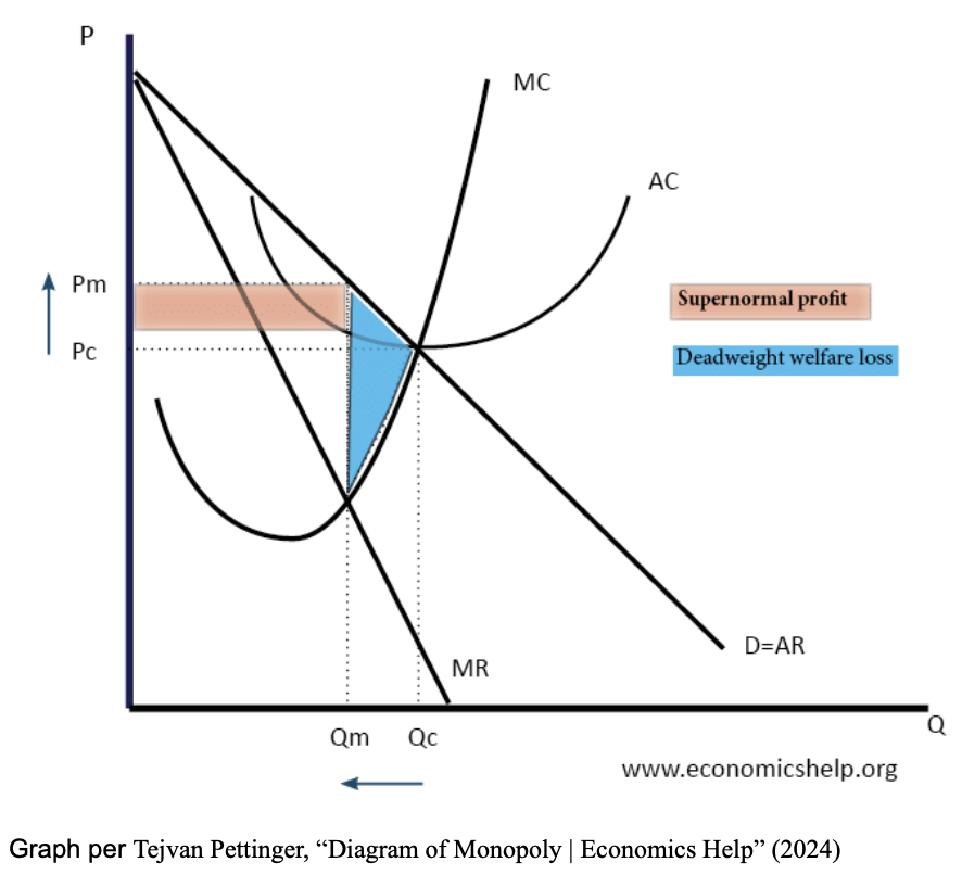
Marginal revenue (MR) is downward sloping because prices need to be decreased to generate additional sales. (Tuovila)
Average Cost (AC) average cost incurred by a firm to produce goods (U shaped!)
Marginal Cost (MC) the cost incurred to produce one extra unit.
Average Revenue = Demand (D=AR) revenue received.
Per Economics Help A-Level (2025), if this market were competitive, price would be Pc and quantity would be Qc. However, in a monopoly, it has market power- it can set quantity at Qm and price at Pm- a quantity that is lower and a price that is higher.
Thus, profit max is where MR = MC, but they charge at Pm. How much profit does the monopoly make? Profit = Q(AR-AC), thus the average revenue is greater than the average cost. The profit is the red section.
The blue section shows the transactions that would happen in a competitive market but don’t happen under a monopoly. The triangle shows the combined loss from producer and consumer surplus (compared to a competitive market). It is the difference between marginal cost -> average revenue and the monopolies’ quantity. (Economics Help A-Level )
This diagram shows that a monopoly is very inefficient because the price is set significantly higher than the marginal cost. (Tejvan Pettinger, “Diagram of Monopoly | Economics Help”)